Simulate an Envirome with a Known Relationship to an Environment Correlation

Core simulator. Given a target correlation \(C_{env}\) among environments, it builds a \(q \times n_{var}\) covariable matrix \(W\) whose environmental kernel recovers a known share of \(C_{env}\). It answers: if the true similarity among my environments is \(C_{env}\), what would an envirome of this size and quality look like, and how much of that similarity would it recover? Pairs with sim_met.

Usage

sim_W(
  C_env,
  noise = 0,
  n_var = 50,
  collinearity = 0,
  n_blocks = 1,
  calibrate = TRUE,
  cal.nrep = 15L,
  marginal = c("gaussian", "right-skewed", "heavy-tailed", "bounded"),
  kernel = c("linear", "rbf"),
  bandwidth = NULL,
  na.frac = 0,
  family.sizes = NULL,
  var_names = NULL,
  env_names = NULL,
  seed = NULL,
  verbose = TRUE
)

Arguments

C_env

q x q correlation AMONG ENVIRONMENTS, from any source (e.g. sim_met$C_env, env_cor, cov2cor(env_kernel(W)$envCov), or hand-specified). NOT a kinship.

noise

numeric in [0, 1]. With calibrate = TRUE, the expected off-diagonal correlation between the simulated kernel and C_env is 1 - noise.

n_var

integer. Number of covariables (columns of \(W\)).

collinearity

numeric in [0, 1). Share of columns collapsed onto drivers (also the within-family strength when family.sizes is used).

n_blocks

integer. Collinear columns grouped into this many families.

calibrate

logical. Solve for the internal variance share \(a\) numerically so noise is on the outcome scale. Default TRUE.

cal.nrep

integer. Monte-Carlo replicates used during calibration.

marginal

character. Marginal distribution of the covariables: "gaussian" (default), "right-skewed", "heavy-tailed" or "bounded". Applied rank-preserving, so recovery is barely changed.

kernel

character. Environmental kernel: "linear" (default, \(WW^\top\)) or "rbf" (Gaussian).

bandwidth

numeric or NULL. RBF bandwidth; NULL uses the median heuristic.

na.frac

numeric in [0, 1). Fraction of entries set to NA in the returned \(W\) (truth is computed on the complete matrix first).

family.sizes

integer vector (optionally named). Column counts per covariable family; must sum to n_var. Overrides n_blocks redundancy and names the columns by family.

var_names, env_names

character. Optional names for columns / rows.

seed

integer. RNG seed. The caller's RNG stream is restored on exit.

verbose

logical. Print a summary. Default TRUE.

Value

A \(q \times n_{var}\) matrix of class "sim_W". Attributes: "C_env" (the target), "K_W" (the realised kernel) and "explained" (a list with r, r2, per-PC variance shares, effective rank eff_rank, the internal share a_internal, the marginal/kernel/na.frac used, and the requested/target values).

Details

Construction. With \(C_{env}^{1/2}\) the symmetric PSD square root of the target, an orthonormal driver \(O\) (\(q\times n_{var}\)) and iid noise \(E\), $$W = \sqrt{1-a}\; C_{env}^{1/2} O \; + \; \sqrt{a}\; E,$$ and the environmental kernel follows the env_kernel convention $$K_W = \frac{W W^{\top}}{\mathrm{tr}(W W^{\top})/q}.$$ Recovery is measured by the off-diagonal Pearson correlation \(r = \mathrm{cor}\big(\mathrm{offdiag}(K_W),\, \mathrm{offdiag}(C_{env})\big)\).

Calibration. When calibrate = TRUE, noise is on the outcome scale: the internal variance share \(a\) is solved by uniroot so that \(E[r] = 1 - \mathrm{noise}\). Because \(r\) decreases in \(a\), noise = 0 gives \(a = 0\) (full recovery) and noise = 1 gives \(a = 1\) (pure noise).

Collinearity. With collinearity > 0, a share of columns is collapsed onto n_blocks driver families, mimicking the redundancy of real enviromes and lowering the effective rank.

C_env is an environment correlation, not a kinship. It must be \(q\times q\) with unit diagonal. Passing a genomic kinship is rejected.

Realism knobs. marginal maps each covariable to a non-Gaussian shape (rank-preserving), kernel = "rbf" builds a Gaussian instead of a linear kernel, family.sizes groups columns into named covariable families (as in real enviromes), and na.frac injects missing values into the returned \(W\) after the truth is computed, so downstream cleaning (e.g. W_matrix imputation) can be tested against a known answer.

References

Costa-Neto, G., et al. (2023). Envirome-wide associations enhance multi-environment prediction. G3 13(2), jkac313.

See also

sim_met, sim_met_C, sim_W_grid, env_cor, env_kernel

Examples

# \donttest{
C <- sim_met_C(q = 10, min.cor = 0.2, max.cor = 0.8, seed = 1)
#> Warning: Rejection sampling failed in 200 tries; C was repaired by eigenvalue clamping.
#>   Requested off-diagonal range [0.200, 0.800]; realised [0.235, 0.712].

## 1. An envirome that recovers ~70% of C (noise is on the outcome scale)
W <- sim_W(C, noise = 0.3, n_var = 50, seed = 1)
#> <sim_W>
#>   environments x covariables . 10 x 50
#>   r(K_W, C_env) off-diagonal . 0.8001   (target 0.7000)
#>   r2  % of env relatedness ... 64.0%
#>   effective rank ............. 7.14 of 50 covariables
#>   PC1 share .................. 20.6%
#>   internal variance share a .. 0.0868
#>   marginal / kernel .......... gaussian / linear
attr(W, "explained")$r
#> [1] 0.800051

## 2. Perfect vs pure-noise enviromes
W_good  <- sim_W(C, noise = 0.0, n_var = 50)
#> <sim_W>
#>   environments x covariables . 10 x 50
#>   r(K_W, C_env) off-diagonal . 1.0000   (target 1.0000)
#>   r2  % of env relatedness ... 100.0%
#>   effective rank ............. 5.84 of 50 covariables
#>   PC1 share .................. 24.6%
#>   internal variance share a .. 0.0000
#>   marginal / kernel .......... gaussian / linear
W_noise <- sim_W(C, noise = 1.0, n_var = 50)
#> <sim_W>
#>   environments x covariables . 10 x 50
#>   r(K_W, C_env) off-diagonal . -0.0776   (target 0.0000)
#>   r2  % of env relatedness ... 0.6%
#>   effective rank ............. 7.36 of 50 covariables
#>   PC1 share .................. 22.2%
#>   internal variance share a .. 1.0000
#>   marginal / kernel .......... gaussian / linear

## 3. Redundant envirome: many collinear columns, low effective rank
W <- sim_W(C, noise = 0.3, n_var = 200, collinearity = 0.8, n_blocks = 5)
#> Warning: Calibration failed; using noise as the raw variance share.
#> <sim_W>
#>   environments x covariables . 10 x 200
#>   r(K_W, C_env) off-diagonal . 0.1501   (target 0.7000)
#>   r2  % of env relatedness ... 2.3%
#>   effective rank ............. 8.54 of 200 covariables
#>   PC1 share .................. 15.2%
#>   internal variance share a .. 0.3000
#>   marginal / kernel .......... gaussian / linear

## 4. Non-Gaussian covariables (rank-preserving marginal transform)
W <- sim_W(C, noise = 0.3, n_var = 60, marginal = "right-skewed")
#> Warning: Calibration failed; using noise as the raw variance share.
#> <sim_W>
#>   environments x covariables . 10 x 60
#>   r(K_W, C_env) off-diagonal . 0.2371   (target 0.7000)
#>   r2  % of env relatedness ... 5.6%
#>   effective rank ............. 7.77 of 60 covariables
#>   PC1 share .................. 18.5%
#>   internal variance share a .. 0.3000
#>   marginal / kernel .......... right-skewed / linear
W <- sim_W(C, noise = 0.3, n_var = 60, marginal = "heavy-tailed")
#> <sim_W>
#>   environments x covariables . 10 x 60
#>   r(K_W, C_env) off-diagonal . 0.7213   (target 0.7000)
#>   r2  % of env relatedness ... 52.0%
#>   effective rank ............. 7.04 of 60 covariables
#>   PC1 share .................. 20.1%
#>   internal variance share a .. 0.0353
#>   marginal / kernel .......... heavy-tailed / linear
W <- sim_W(C, noise = 0.3, n_var = 60, marginal = "bounded")
#> Warning: Calibration failed; using noise as the raw variance share.
#> <sim_W>
#>   environments x covariables . 10 x 60
#>   r(K_W, C_env) off-diagonal . -0.2372   (target 0.7000)
#>   r2  % of env relatedness ... 5.6%
#>   effective rank ............. 7.75 of 60 covariables
#>   PC1 share .................. 19.3%
#>   internal variance share a .. 0.3000
#>   marginal / kernel .......... bounded / linear

## 5. Gaussian RBF kernel instead of the linear WW'
W <- sim_W(C, noise = 0.3, n_var = 60, kernel = "rbf")
#> <sim_W>
#>   environments x covariables . 10 x 60
#>   r(K_W, C_env) off-diagonal . 0.8003   (target 0.7000)
#>   r2  % of env relatedness ... 64.0%
#>   effective rank ............. 6.95 of 60 covariables
#>   PC1 share .................. 22.2%
#>   internal variance share a .. 0.0770
#>   marginal / kernel .......... gaussian / rbf
W <- sim_W(C, noise = 0.3, n_var = 60, kernel = "rbf", bandwidth = 2)
#> <sim_W>
#>   environments x covariables . 10 x 60
#>   r(K_W, C_env) off-diagonal . 0.5236   (target 0.7000)
#>   r2  % of env relatedness ... 27.4%
#>   effective rank ............. 6.89 of 60 covariables
#>   PC1 share .................. 22.8%
#>   internal variance share a .. 0.0688
#>   marginal / kernel .......... gaussian / rbf

## 6. Inject missing values AFTER the truth is computed
W <- sim_W(C, noise = 0.3, n_var = 60, na.frac = 0.1)
#> <sim_W>
#>   environments x covariables . 10 x 60
#>   r(K_W, C_env) off-diagonal . 0.6721   (target 0.7000)
#>   r2  % of env relatedness ... 45.2%
#>   effective rank ............. 6.84 of 60 covariables
#>   PC1 share .................. 25.2%
#>   internal variance share a .. 0.0865
#>   marginal / kernel .......... gaussian / linear
#>   missing values injected .... 10.0%
sum(is.na(W))
#> [1] 60

## 7. Named covariable families (sizes must sum to n_var)
W <- sim_W(C, n_var = 12, family.sizes = c(temp = 4, rain = 5, rad = 3))
#> <sim_W>
#>   environments x covariables . 10 x 12
#>   r(K_W, C_env) off-diagonal . 0.3512   (target 1.0000)
#>   r2  % of env relatedness ... 12.3%
#>   effective rank ............. 2.68 of 12 covariables
#>   PC1 share .................. 53.5%
#>   internal variance share a .. 0.0000
#>   marginal / kernel .......... gaussian / linear
colnames(W)
#>  [1] "temp_1" "temp_2" "temp_3" "temp_4" "rain_1" "rain_2" "rain_3" "rain_4"
#>  [9] "rain_5" "rad_1"  "rad_2"  "rad_3" 

## 8. Custom names and a faster/looser calibration
W <- sim_W(C, noise = 0.4, n_var = 30, cal.nrep = 5,
           env_names = paste0("Loc", 1:10),
           var_names = paste0("bio", 1:30), seed = 1)
#> <sim_W>
#>   environments x covariables . 10 x 30
#>   r(K_W, C_env) off-diagonal . 0.4270   (target 0.6000)
#>   r2  % of env relatedness ... 18.2%
#>   effective rank ............. 6.86 of 30 covariables
#>   PC1 share .................. 22.7%
#>   internal variance share a .. 0.1438
#>   marginal / kernel .......... gaussian / linear

## 9. Raw (uncalibrated) internal variance share
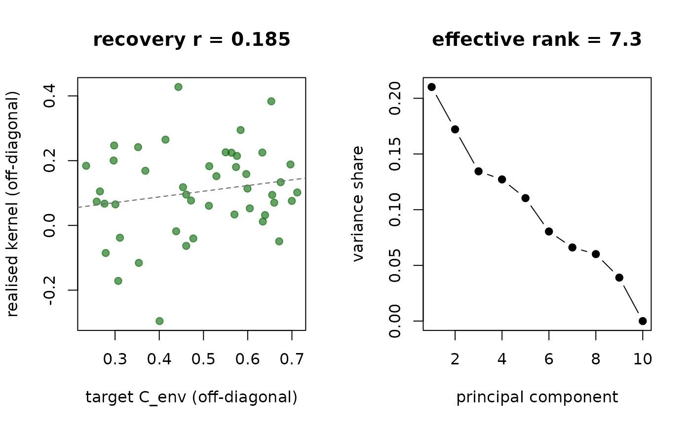
W <- sim_W(C, noise = 0.5, n_var = 50, calibrate = FALSE)
#> <sim_W>
#>   environments x covariables . 10 x 50
#>   r(K_W, C_env) off-diagonal . 0.1849   (target 0.5000)
#>   r2  % of env relatedness ... 3.4%
#>   effective rank ............. 7.34 of 50 covariables
#>   PC1 share .................. 21.0%
#>   internal variance share a .. 0.5000
#>   marginal / kernel .......... gaussian / linear
plot(W)

# }