EnvRtype: Envirotyping for Quantitative Genetics and Plant Breeding

Germano Costa-Neto¹
Fernanda G. Pontes²

Created 12 August 2026 · Revised 22 October 2026

EnvRtype is an enviromics toolkit for genotype-by-environment (GxE) analysis and envirotype-informed genomic prediction. From geographic coordinates and date ranges it collects worldwide weather, soil, elevation, bioclimatic and CMIP6 climate-scenario data, derives agro-meteorological parameters and a FAO-56 soil water balance, maps daily weather onto crop developmental stages, and builds environmental covariable matrices, envirotype typologies, mega-environment clusters and relatedness kernels. It then fits Bayesian reaction-norm kernel models to predict trained genotypes at untested locations and planting dates, with coverage diagnostics, spatial mapping and planting-window optimisation. A simulation engine generates multi-environment trials and enviromes with known genetic architecture to validate every layer.

This vignette walks through the whole package, section by section, following the four data layers plus the simulation engine.

library(EnvRtype)

Why envirotyping

A breeder evaluating 500 hybrids across 30 locations observes that rankings change from site to site. Classical quantitative genetics treats this genotype-by-environment interaction as a variance component to be estimated and, usually, discarded:

$$y_{ij} = \mu + g_i + e_j + (ge)_{ij} + \varepsilon_{ij}$$

The term $(ge)_{ij}$ absorbs everything specific to hybrid $i$ in location $j$. It is estimable only where that combination was actually planted, so it cannot be transferred to a new site, a new season, or a new planting date. Every untested combination is a blank.

Envirotyping replaces the label $e_j$ with a description. Let $\mathbf{w}_j \in \mathbb{R}^k$ be a vector of $k$ measured environmental quantities at site $j$ — mean temperature during flowering, accumulated water deficit during grain fill, radiation at emergence. The interaction then becomes a function of measurable covariates rather than an unstructured effect:

$$y_{ij} = \mu + g_i + \mathbf{w}_j^{\top}\boldsymbol{\beta} + \sum_{m=1}^{k} g_{im}\, w_{jm} + \varepsilon_{ij}$$

This is a reaction norm: genotype $i$ has its own slope $g_{im}$ against each environmental gradient $m$. Because $\boldsymbol{\beta}$ and the slopes are indexed by covariable, not by site, they carry to any location where $\mathbf{w}$ can be computed — which, for weather and soil data, is anywhere on Earth.

That single substitution is what makes prediction into unplanted environments possible, and it is the organising idea behind every function in this package.

From covariables to kernels

Fitting $k$ separate slopes per genotype is infeasible when $k$ is in the hundreds and environments number in the tens. The standard remedy is to work with relatedness rather than with individual coefficients. Define the environmental kinship

$$\mathbf{K}_E = \frac{\mathbf{W}\mathbf{W}^{\top}}{\mathrm{tr}(\mathbf{W}\mathbf{W}^{\top})/q}$$

for $q$ environments, exactly analogous to the genomic relationship matrix of VanRaden (2008). Two environments are “related” to the degree their covariable profiles align. The model becomes

$$\mathbf{y} = \mathbf{1}\mu + \mathbf{Z}_g\mathbf{g} + \mathbf{Z}_e\mathbf{e} + \mathbf{g}\!\otimes\!\mathbf{e} + \boldsymbol{\varepsilon}, \qquad \mathbf{g} \sim N(\mathbf{0}, \mathbf{K}_G\sigma_g^2), \quad \mathbf{e} \sim N(\mathbf{0}, \mathbf{K}_E\sigma_e^2)$$

with the GxE term given a Hadamard product $\mathbf{K}_G \circ \mathbf{K}_E$. The number of parameters no longer grows with $k$, and prediction at a new site requires only its row in $\mathbf{K}_E$ — computable from downloaded weather without a single phenotype.

Why the growing season must be partitioned

A season-long mean is close to useless. Maize is largely indifferent to heat during vegetative growth and acutely sensitive during the two weeks around anthesis; averaging over 120 days dilutes the flowering signal into noise. So every characterisation function in this package accepts by.interval = TRUE with a time.window, producing covariables indexed by factor × stage rather than by factor alone.

The cost is dimensionality: 17 weather factors across 51 three-day intervals gives 867 indices for 9 environments (Della Coletta et al. 2023). Those indices are heavily collinear by construction, which is what env_pca() exists to handle.

How the package is organised

Layer	Purpose	Key functions
1 · Acquire	Pull weather, soil and geodata	get_weather(), get_soil(), get_elevation()
2 · Process	Derive agro-meteorological parameters	processWTH(), water_balance(), env_phenology()
3 · Characterise	Build covariables, typologies, indices	W_matrix(), env_typing(), env_pca()
4 · Model & scan	Kernels, prediction, untested environments	get_kernel(), kernel_model(), scan_untested_envs()
Simulate	Ground truth to validate every layer	sim_met(), sim_W()

Layers 1 and 2 require network access, so those chunks are shown but not evaluated. Everything from layer 3 onward runs on the bundled HELIX maize data and executes in full.

data(maizeWTH)
data(maizeYield)
data(maizeG)

dim(maizeWTH)
#> [1] 756  30
dim(maizeYield)
#> [1] 750   3
dim(maizeG)
#> [1] 150 150

maizeWTH holds daily weather for five Brazilian sites; maizeYield holds grain yield for 150 hybrids in those five environments; maizeG is the genomic relationship matrix.

---

1 · Data acquisition

Weather comes from NASA POWER through nasapower; soil from SoilGrids 2.0; elevation and bioclimate from WorldClim 2; agro-ecological zones from GAEZ v4; future scenarios from CMIP6.

Daily weather

env   <- c("NAIROBI", "NAKURU", "ELDORET")
lat   <- c(-1.28, -0.30, 0.52)
lon   <- c(36.82, 36.08, 35.27)
start <- rep("2020-03-01", 3)
end   <- rep("2020-07-31", 3)

wth <- get_weather(env.id = env, lat = lat, lon = lon,
                   start.day = start, end.day = end)

get_weather() accepts parallel = TRUE with workers, chunks long date ranges via chunk_size, and retries failed calls tries times with sleep seconds between attempts.

Hourly weather, day/night partitioned

wth_h <- get_weather_hourly(env.id = env, lat = lat, lon = lon,
                            start.day = start, end.day = end)

This is a separate function rather than an argument on get_weather() because POWER caps hourly requests at 15 parameters, and T2M_MAX, T2M_MIN and FROST_DAYS are daily aggregates that do not exist hourly. It returns one row per environment-day with day, night and pre-dawn partitions.

Note the limitation: POWER hourly is MERRA-2 reanalysis, not observation. The diurnal cycle is modelled.

Resumable downloads

Large multi-environment downloads fail partway through. The resumable variants checkpoint to disk:

wth <- get_weather_resumable(env.id = env, lat = lat, lon = lon,
                             start.day = start, end.day = end,
                             run.id = "kenya2020")

read_progress_log("kenya2020")           # what succeeded, what failed
wth <- restart_from_log("kenya2020")     # resume, retrying failures

get_soil_resumable() does the same for soil.

Soil, elevation, bioclimate and zones

soil <- get_soil(env.id = env, lat = lat, lon = lon)
elev <- get_elevation(env.id = env, lat = lat, lon = lon)
bioc <- get_bioclim(env.id = env, lat = lat, lon = lon, vars = 1:19)
aez  <- get_AEZ(env.id = env, lat = lat, lon = lon)

For future projections:

fut <- get_climate_scenario(env.id = env, lat = lat, lon = lon,
                            scenario = "ssp245")

Raster extraction at trial coordinates uses get_spatial().

---

2 · Processing

Agro-meteorological parameters

Raw POWER output gives temperature, radiation and precipitation. What matters agronomically are derived quantities. processWTH() computes all of them:

maizeWTH <- processWTH(env.data = maizeWTH, verbose = FALSE)
names(maizeWTH)
#>  [1] "env"               "LON"               "LAT"              
#>  [4] "YEAR"              "MM"                "DD"               
#>  [7] "DOY"               "YYYYMMDD"          "T2M"              
#> [10] "T2M_MAX"           "T2M_MIN"           "PRECTOT"          
#> [13] "WS2M"              "RH2M"              "T2MDEW"           
#> [16] "ALLSKY_SFC_LW_DWN" "ALLSKY_SFC_SW_DWN" "ALLSKY_TOA_SW_DWN"
#> [19] "daysFromStart"     "SRAD"              "n"                
#> [22] "N"                 "RTA"               "VPD"              
#> [25] "SPV"               "ETP"               "PETP"             
#> [28] "GDD"               "FRUE"              "T2M_RANGE"

Three derived columns carry most of the signal:

Column	Meaning
GDD	Growing degree days — thermal time
FRUE	Temperature effect on radiation use efficiency, in [0, 1]
PETP	Precipitation minus potential evapotranspiration; negative = deficit

head(maizeWTH[, c("env", "daysFromStart", "GDD", "FRUE", "PETP")])
#>   env daysFromStart    GDD      FRUE      PETP
#> 1  NM             1 15.855 0.9326471 -8.602829
#> 2  NM             2 16.735 0.9844118 -5.695403
#> 3  NM             3 16.390 0.9641176 -3.869658
#> 4  NM             4 15.780 0.9282353  1.352827
#> 5  NM             5 14.480 0.8517647 11.364616
#> 6  NM             6 15.140 0.8905882  5.279136

The three param_* functions run individually if you want finer control:

d <- param_radiation(env.data = maizeWTH, merge = TRUE)
d <- param_atmospheric(env.data = d, Alt = 600)
d <- param_temperature(env.data = d, Tbase1 = 9, Tbase2 = 45,
                       Topt1 = 26, Topt2 = 32)

Setting method = "legacy" in processWTH() reproduces the 2021 behaviour.

Summarising by environment or stage

sm <- summaryWTH(env.data = maizeWTH, env.id = "env",
                 days.id = "daysFromStart",
                 var.id = c("T2M", "PRECTOT", "FRUE"),
                 verbose = FALSE)
head(sm)
#>   env variable       mean       sum  prob_0.25   prob_0.5  prob_0.75
#> 1  IP     FRUE  0.8681976  142.3844  0.8120588  0.8698529  0.9383088
#> 2  IP  PRECTOT  2.7785976  455.6900  0.0175000  0.3900000  3.2925000
#> 3  IP      T2M 23.2651829 3815.4900 22.1375000 23.2550000 24.5950000
#> 4  NM     FRUE  0.9471367  128.8106  0.9208088  0.9483824  0.9810294
#> 5  NM  PRECTOT  2.8254412  384.2600  0.0100000  1.0100000  3.6775000
#> 6  NM      T2M 24.7127941 3360.9400 24.2875000 24.7800000 25.1925000

Split the season into developmental intervals:

stages   <- c("VE", "V1_V6", "V6_VT", "VT_R1")
interval <- c(0, 7, 30, 65, 90)

sm_stage <- summaryWTH(env.data = maizeWTH, env.id = "env",
                       days.id = "daysFromStart",
                       var.id = c("FRUE", "PETP"),
                       by.interval = TRUE,
                       time.window = interval,
                       names.window = stages,
                       verbose = FALSE)
head(sm_stage)
#>   env    interval variable       mean        sum  prob_0.25   prob_0.5
#> 1  IP Interval_90     FRUE  0.8146706   61.10029  0.7775000  0.8150000
#> 2  IP Interval_90     PETP -5.2008800 -374.46336 -6.3073859 -5.8348478
#> 3  IP       V1_V6     FRUE  0.9354987   21.51647  0.9152941  0.9394118
#> 4  IP       V1_V6     PETP -1.4631906  -33.65338 -7.1046784 -3.6571826
#> 5  IP       V6_VT     FRUE  0.9131092   31.95882  0.8805882  0.9252941
#> 6  IP       V6_VT     PETP -1.4355421  -50.24397 -5.5428601 -2.3442705
#>    prob_0.75
#> 1  0.8520588
#> 2 -4.9447235
#> 3  0.9598529
#> 4  1.1608272
#> 5  0.9561765
#> 6  1.1272337

A season-long mean hides stress concentrated around flowering. Stage resolution is almost always the more informative view.

Phenology

env_phenology() converts thermal time into developmental stages:

show_phenology("maize")        # inspect the bundled template
phenology_templates()          # all available crops

ph <- env_phenology(env.data = maizeWTH, env.id = "env",
                    day.id = "daysFromStart",
                    crop = "maize", method = "gdd")

Three thermal-time methods are available: "gdd" (simple), "baskerville" (sine-wave correction for days crossing the base temperature), and "trapezoid". Photoperiod sensitivity is enabled with photoperiod = TRUE.

FAO-56 water balance

Combining weather with soil hydraulic properties gives a daily root-zone water balance:

wb <- water_balance(env.data = maizeWTH, soil.data = soil,
                    env.id = "env", days.id = "daysFromStart",
                    PREC = "PRECTOT",
                    root.depth = 1000, root.init = 300,
                    dap.root.max = 60)

summary_water_balance(wb, by.interval = TRUE,
                      time.window = interval,
                      names.window = stages)

Read the scope limits before drawing agronomic conclusions. This is the FAO-56 single coefficient method. It does not separate soil evaporation from transpiration, does not model runoff — all rainfall is assumed to infiltrate — and does not model capillary rise or lateral flow. On crusted or steep soils the no-runoff assumption overestimates stored water and therefore underestimates stress. The default Kc and p values describe a generic 120-day maize crop and are tabulated starting points, not calibrated values.

---

3 · Characterisation

The environmental covariable matrix

W has environments in rows and covariables in columns — the numeric representation every downstream model needs.

W <- W_matrix(env.data = maizeWTH,
              var.id = c("FRUE", "PETP", "T2M_MAX", "T2M_MIN"),
              statistic = "mean",
              verbose = FALSE)
dim(W)
#> [1] 5 4
round(W[, 1:4], 2)
#>    FRUE_mean PETP_mean T2M_MAX_mean T2M_MIN_mean
#> NM      0.73     -0.04         0.21         0.82
#> SO      1.11     -1.30         1.48         1.15
#> PM     -0.61     -0.27        -0.52        -0.71
#> IP      0.13      0.11         0.05        -0.04
#> SE     -1.36      1.49        -1.23        -1.22

Stage-resolved, which separates flowering stress from vegetative stress:

W_stage <- W_matrix(env.data = maizeWTH,
                    var.id = c("FRUE", "PETP"),
                    by.interval = TRUE,
                    time.window = interval,
                    names.window = stages,
                    verbose = FALSE)
dim(W_stage)
#> [1]  5 10
colnames(W_stage)
#>  [1] "FRUE_mean_VE"          "FRUE_mean_V1_V6"       "FRUE_mean_V6_VT"      
#>  [4] "FRUE_mean_VT_R1"       "FRUE_mean_Interval_90" "PETP_mean_VE"         
#>  [7] "PETP_mean_V1_V6"       "PETP_mean_V6_VT"       "PETP_mean_VT_R1"      
#> [10] "PETP_mean_Interval_90"

Two covariables across four stages gives eight columns, each with its own coefficient downstream. W_matrix() centres and scales by default; QC = TRUE activates sd.tol filtering; impute handles missing values.

Environmental typologies

A covariable says how much; an envirotype says what kind. Where crop physiology defines meaningful thresholds, discretising at those thresholds is more informative than a mean, because it preserves the shape of the exposure distribution rather than collapsing it.

For temperature, the cardinals are $T_b$ (base, below which development stops), $T_{o1}$ and $T_{o2}$ (the optimum band) and $T_c$ (critical/lethal). Counting the proportion of days falling in each band gives a frequency profile:

$$f_{jc} = \frac{1}{n_j}\sum_{d=1}^{n_j} \mathbb{1}\{x_{jd} \in \text{class } c\}$$

Two sites with identical mean temperature can have completely different profiles — one steady at the optimum, the other oscillating between cold nights and lethal afternoons. The mean cannot distinguish them; the typology can.

Supply cardinals when the crop physiology is known — maize temperature: base 0 °C, lower optimum 9 °C, upper optimum 32 °C, lethal 45 °C.

card_temp <- c( 9, 32, 45,Inf)

ET <- env_typing(env.data = maizeWTH, var.id = "T2M", env.id = "env",
                 cardinals = card_temp, verbose = FALSE)
head(ET)
#>      env.variable Freq env       interval var
#> 1 T2M_(22.8,23.2]    5  NM by environment T2M
#> 2 T2M_(23.2,23.6]    4  NM by environment T2M
#> 3 T2M_(23.6,23.9]    8  NM by environment T2M
#> 4 T2M_(23.9,24.3]   26  NM by environment T2M
#> 5 T2M_(24.3,24.7]   22  NM by environment T2M
#> 6 T2M_(24.7,25.1]   28  NM by environment T2M

Without cardinals, classes are cut at observed quantiles:

ET_rain <- env_typing(env.data = maizeWTH, var.id = "PRECTOT",
                      env.id = "env", verbose = FALSE)
head(ET_rain)
#>          env.variable Freq env       interval     var
#> 1    PRECTOT_(0,0.28]   23  NM by environment PRECTOT
#> 2 PRECTOT_(0.28,2.88]   34  NM by environment PRECTOT
#> 3 PRECTOT_(2.88,23.8]   45  NM by environment PRECTOT
#> 4    PRECTOT_(0,0.28]   23  PM by environment PRECTOT
#> 5 PRECTOT_(0.28,2.88]   41  PM by environment PRECTOT
#> 6 PRECTOT_(2.88,23.8]   31  PM by environment PRECTOT

Data-driven envirotype mining is available via envirotype_mining = TRUE, which selects the number of classes by silhouette over k.range. Joint typologies across variables use joint = TRUE.

The envirotype frequency matrix

T_matrix() returns environments by envirotype frequency — rows are normalised compositions:

Tm <- T_matrix(env.data = maizeWTH, var.id = "T2M", env.id = "env",
               cardinals = card_temp, verbose = FALSE)
dim(Tm)
#> [1]  5 45

Because rows are already normalised, pass is.scaled = TRUE when feeding a T_matrix to env_kernel().

Clustering environments into mega-environments

A mega-environment is a repeatable group of locations that rank genotypes similarly. If such groups exist, a breeding programme can select within each rather than chasing a single genotype that wins everywhere — which usually does not exist.

env_cluster() approximates them by grouping environments with similar enviromic profiles. The number of clusters is chosen by maximising the average silhouette width

$$s(i) = \frac{b(i) - a(i)}{\max\{a(i),\, b(i)\}}$$

where $a(i)$ is the mean distance from environment $i$ to others in its own cluster and $b(i)$ the mean distance to the nearest other cluster. Values near 1 mean well-separated groups; values near 0 mean the boundary is arbitrary.

cl <- env_cluster(W = W, k.max = 4, seed = 1234, verbose = FALSE)
cl$k
#> [1] 2
cl$clusters
#> NM SO PM IP SE 
#>  2  2  1  2  1

Inspect the silhouette profile before trusting the chosen k:

cl$silhouette
#>   k avg.silhouette
#> 1 2      0.3135561
#> 2 3      0.2012617
#> 3 4      0.1054217

If the best average width is below roughly 0.25, the data do not support discrete mega-environments and a continuous reaction-norm treatment is more honest than forcing groups.

The environment kinship implied by the clustering is returned too:

round(cl$env.kinship, 2)
#>       NM    SO    PM    IP    SE
#> NM  1.00  0.67 -0.94 -0.43 -0.77
#> SO  0.67  1.00 -0.86 -0.42 -0.99
#> PM -0.94 -0.86  1.00  0.58  0.91
#> IP -0.43 -0.42  0.58  1.00  0.38
#> SE -0.77 -0.99  0.91  0.38  1.00

Forcing a fixed number of groups:

cl2 <- env_cluster(W = W, k = 2, seed = 1234, verbose = FALSE)
table(cl2$clusters)
#> 
#> 1 2 
#> 3 2

Five environments is a small illustration; the method is intended for TPE surveys with tens to hundreds of sites.

Which environmental factors drive a grouping

env_cluster() is unsupervised — it groups by enviromic profile alone. env_target_importance() is its supervised counterpart: environments are grouped by what the breeder cares about (yield level, heritability, selection accuracy), and the enviromic data are then asked to explain that grouping via a Random Forest.

The target Y is an environment-level quantity — one value per environment, not the raw plot data:

Y_env <- tapply(maizeYield$value, maizeYield$env, mean)
Y_env <- Y_env[rownames(W)]
round(Y_env, 3)
#>     NM     SO     PM     IP     SE 
#> -0.556  0.919  0.838 -1.079  0.165

if (requireNamespace("randomForest", quietly = TRUE)) {
  imp <- env_target_importance(Y = Y_env, W = W, k = 2, ntree = 200,
                               seed = 1234, verbose = FALSE)
  print(imp$k)
  print(imp$clusters)
  head(imp$importance)
}
#> [1] 2
#> NM SO PM IP SE 
#>  1  2  2  1  2
#>       variable importance
#> 1    PETP_mean     0.5965
#> 2 T2M_MAX_mean     0.5225
#> 3 T2M_MIN_mean     0.4955
#> 4    FRUE_mean     0.4695

Variables at the top of $importance are candidate drivers of the observed stratification — the environmental factors worth measuring in future trials, or worth targeting with stress-tolerance breeding.

A multi-trait target works too. Here environments are grouped by both mean yield and within-environment variability:

if (requireNamespace("randomForest", quietly = TRUE)) {
  Ymat <- cbind(
    mean = Y_env,
    sd   = tapply(maizeYield$value, maizeYield$env, stats::sd)[rownames(W)]
  )
  imp2 <- env_target_importance(Y = Ymat, W = W, k = 2, ntree = 200,
                                seed = 1234, verbose = FALSE)
  head(imp2$importance)
}
#>       variable importance
#> 1    PETP_mean  0.6498333
#> 2 T2M_MAX_mean  0.5183333
#> 3 T2M_MIN_mean  0.4910000
#> 4    FRUE_mean  0.4488333

Use importance.type = "permutation" when covariables differ in scale or cardinality — MeanDecreaseGini is biased towards high-cardinality predictors.

Multi-year risk profiles and TPE weights

With several years of weather for the same sites, env_risk_profile() gives envirotype frequencies per stage across seasons:

risk <- env_risk_profile(env.data = long_term_wth,
                         site.id = "env", date.id = "YYYYMMDD",
                         var.id = c("T2M", "PETP"),
                         season.length = 150,
                         crop = "maize", by.stage = TRUE)

tpe_weights(risk, stage = "flowering")

Projecting that baseline onto a future scenario:

project_risk(baseline = risk, scenario = fut)

Copula-based indices

env_copula() reparameterises W onto copula scales, separating the marginal behaviour of each covariable from their dependence structure:

cop <- env_copula(W = W, index = "pobs")
#> ---------------------------------------------------------------
#> env_copula -- reparameterises covariables into copula indices
#> Last updated at 09/27/2026
#> ---------------------------------------------------------------
#> Warning: Only 5 environments: copula indices are rank statistics across
#> environments and will be very coarse. Interpret with care.
#> env_copula: 5 environments, 4 covariables, 1 block(s); index = 'pobs'.
dim(cop)
#> [1] 5 4

Options are "pobs", "joint", "survival", "kendall" and "all".

Interval-resolved dissection and PCA

Following Della Coletta et al. (2023), env_indices() builds an environment × (factor × interval) matrix — the paper used 3-day intervals to 151 DAP, giving 51 intervals × 17 factors = 867 indices.

idx <- env_indices(env.data = maizeWTH, env.id = "env",
                   day.id = "daysFromStart",
                   var.id = c("FRUE", "PETP", "T2M"),
                   interval = 10L, end.day = 90L,
                   statistic = "mean", verbose = FALSE)
dim(idx)
#> [1]  5 27

These indices are heavily correlated by construction, which is what PCA is for:

pca <- env_pca(W = idx, scale. = TRUE, verbose = FALSE)
head(pca$variance)
#>    PC       sd       prop       cum
#> 1 PC1 4.253636 0.67012674 0.6701267
#> 2 PC2 1.961418 0.14248742 0.8126142
#> 3 PC3 1.850674 0.12685159 0.9394657
#> 4 PC4 1.278446 0.06053425 1.0000000

The result carries $scores (environment × PC), $loadings (index × PC), $variance (PC, sd, prop, cum), the underlying $prcomp object, $dropped (constant indices removed before scaling) and $meta, which maps each index back to its factor, interval and day:

head(pca$meta)
#>       index factor interval  day
#> 1 FRUE_i001   FRUE     i001  5.5
#> 2 FRUE_i002   FRUE     i002 15.5
#> 3 FRUE_i003   FRUE     i003 25.5
#> 4 FRUE_i004   FRUE     i004 35.5
#> 5 FRUE_i005   FRUE     i005 45.5
#> 6 FRUE_i006   FRUE     i006 55.5
dim(pca$scores)
#> [1] 5 4
dim(pca$loadings)
#> [1] 27  4

env_pca() defaults to scale. = TRUE deliberately. The factors sit on wildly different scales — radiation in MJ/m²/day, precipitation in mm, unitless FRUE in [0,1] — so an unscaled PCA is dominated by whichever has the largest variance. Set scale. = FALSE for a covariance-matrix PCA. Zero-variance indices are dropped before scaling rather than silently producing NaN.

How many PCs to keep is a judgement, not a fixed number:

env_pca_scree(pca, verbose = FALSE)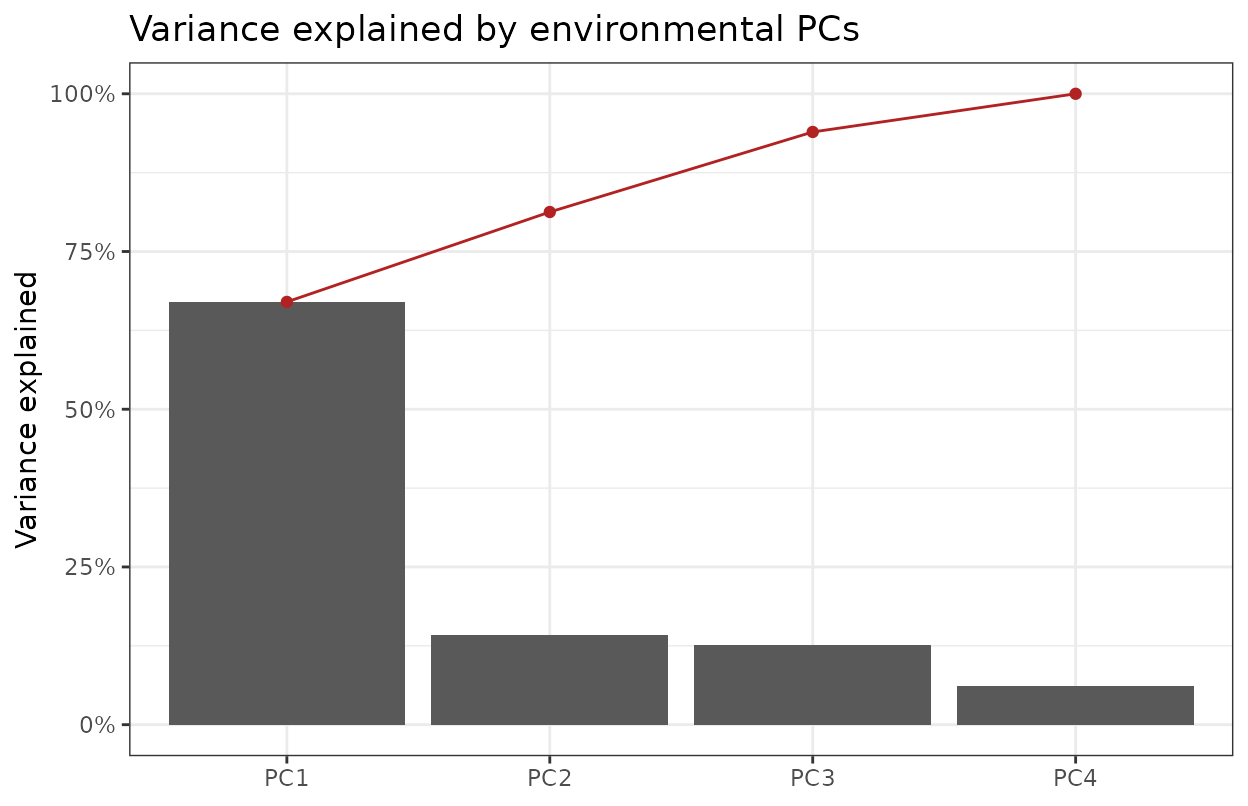

env_pca_biplot(pca, pc = c(1, 2), verbose = FALSE)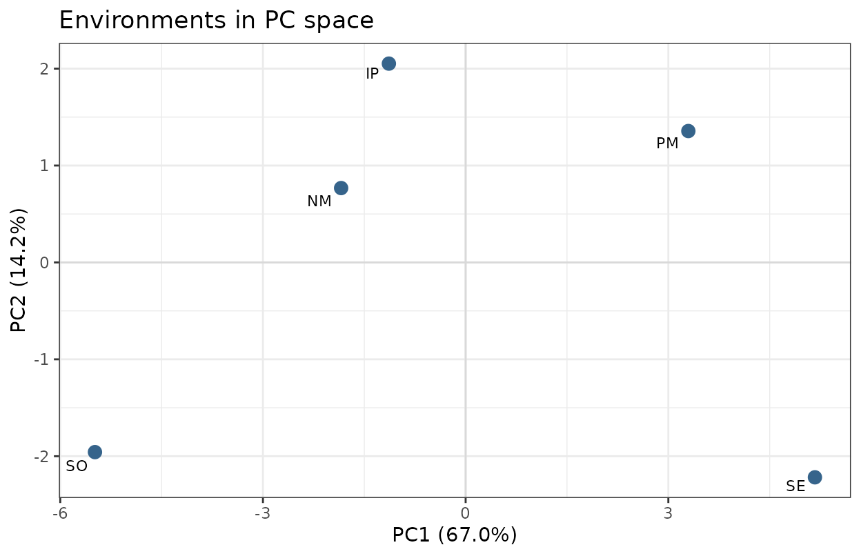

Loadings through the season show which factor at which growth stage drives a component:

env_loading_curve(pca, pc = 1, span = 0.4, verbose = FALSE)
#> Warning in simpleLoess(y, x, w, span, degree = degree, parametric = parametric,
#> : span too small.  fewer data values than degrees of freedom.
#> Warning in simpleLoess(y, x, w, span, degree = degree, parametric = parametric,
#> : pseudoinverse used at 5.1
#> Warning in simpleLoess(y, x, w, span, degree = degree, parametric = parametric,
#> : neighborhood radius 20.4
#> Warning in simpleLoess(y, x, w, span, degree = degree, parametric = parametric,
#> : reciprocal condition number 0
#> Warning in simpleLoess(y, x, w, span, degree = degree, parametric = parametric,
#> : There are other near singularities as well. 416.16
#> Warning in simpleLoess(y, x, w, span, degree = degree, parametric = parametric,
#> : span too small.  fewer data values than degrees of freedom.
#> Warning in simpleLoess(y, x, w, span, degree = degree, parametric = parametric,
#> : pseudoinverse used at 5.1
#> Warning in simpleLoess(y, x, w, span, degree = degree, parametric = parametric,
#> : neighborhood radius 20.4
#> Warning in simpleLoess(y, x, w, span, degree = degree, parametric = parametric,
#> : reciprocal condition number 0
#> Warning in simpleLoess(y, x, w, span, degree = degree, parametric = parametric,
#> : There are other near singularities as well. 416.16
#> Warning in simpleLoess(y, x, w, span, degree = degree, parametric = parametric,
#> : span too small.  fewer data values than degrees of freedom.
#> Warning in simpleLoess(y, x, w, span, degree = degree, parametric = parametric,
#> : pseudoinverse used at 5.1
#> Warning in simpleLoess(y, x, w, span, degree = degree, parametric = parametric,
#> : neighborhood radius 20.4
#> Warning in simpleLoess(y, x, w, span, degree = degree, parametric = parametric,
#> : reciprocal condition number 0
#> Warning in simpleLoess(y, x, w, span, degree = degree, parametric = parametric,
#> : There are other near singularities as well. 416.16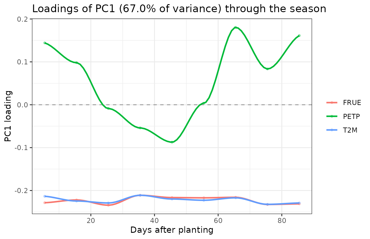

Correlation structure among indices:

env_cor_heatmap(idx, order = "factor", verbose = FALSE)
#> Mean |r| among indices: 0.609  (high values justify the PCA)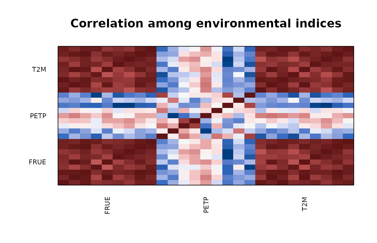

Relating PCs to an external per-environment variable — mean yield, for instance:

env_mean <- tapply(maizeYield$value, maizeYield$env, mean)
env_mean <- env_mean[rownames(pca$scores)]

env_pc_associate(pca, y = env_mean, method = "pearson",
                 p.adjust = "BH", verbose = FALSE)
#>   column  PC           r          p     p.adj n
#> 1     y1 PC3 -0.83607964 0.07767937 0.3107175 5
#> 2     y1 PC2 -0.53714075 0.35057276 0.7011455 5
#> 3     y1 PC4  0.09667016 0.87710771 0.9290825 5
#> 4     y1 PC1  0.05572730 0.92908254 0.9290825 5

A PC that correlates with mean yield identifies an environmental gradient the crop is actually responding to. Combined with env_loading_curve(), which shows which factor at which stage loads on that PC, this is how a vague observation like “site 3 underperformed” becomes “site 3 accumulated water deficit during grain fill”.

Benjamini–Hochberg adjustment is applied by default because one test is run per retained PC.

Soil zoning by Gaussian mixture

zones <- soil_classification(soil.data = soil)

The method follows the standard GMM zoning pipeline with BIC model selection. Texture fractions are compositional, so a log-ratio transform is applied before clustering. Read the documentation note: this is not a byte-for-byte reproduction of Zhang et al. (2025), and SoilGrids carries no heavy metals, so the cadmium application in that paper cannot be reproduced here.

---

4 · Prediction

Environmental relatedness kernels

Two environments with similar conditions should rank genotypes similarly. A kernel turns that intuition into a covariance matrix.

Linear (GB). The environmental analogue of VanRaden’s genomic relationship matrix:

$$\mathbf{K}_E = \frac{\mathbf{W}\mathbf{W}^{\top}} {\mathrm{tr}(\mathbf{W}\mathbf{W}^{\top})/q}$$

The trace normalisation puts the kernel on a scale comparable to $\mathbf{K}_G$, so variance components from the two sources can be read against each other.

Gaussian (GK). Similarity decays nonlinearly with distance:

$$k(\mathbf{w}_i, \mathbf{w}_j) = \exp\!\left(-h\, \frac{\lVert \mathbf{w}_i - \mathbf{w}_j \rVert^2}{q_{50}}\right)$$

where $q_{50}$ is the median squared Euclidean distance, making the bandwidth scale-free. Use this when a doubling of stress does more than double the penalty — common for heat and drought, where damage is threshold-like.

Arc-cosine deep (DK). Emulates an infinitely wide neural network with deep.layers hidden layers (Cuevas et al. 2019), recursively:

$$k^{(l)}(\mathbf{w}_i,\mathbf{w}_j) = \frac{1}{\pi} \sqrt{k^{(l-1)}_{ii} k^{(l-1)}_{jj}} \left(\sin\theta^{(l-1)} + (\pi - \theta^{(l-1)})\cos\theta^{(l-1)}\right)$$

No bandwidth to tune, at the cost of interpretability.

K_lin <- env_kernel(env.data = W, gaussian = FALSE, verbose = FALSE)
round(K_lin$envCov, 2)
#>       NM    SO    PM    IP    SE
#> NM  0.39  0.66 -0.35  0.02 -0.72
#> SO  0.66  2.00 -0.60  0.01 -2.08
#> PM -0.35 -0.60  0.38 -0.03  0.60
#> IP  0.02  0.01 -0.03  0.01 -0.01
#> SE -0.72 -2.08  0.60 -0.01  2.21

K_lin <- env_kernel(env.data = W, gaussian = FALSE, verbose = FALSE)
round(K_lin$envCov, 2)
#>       NM    SO    PM    IP    SE
#> NM  0.39  0.66 -0.35  0.02 -0.72
#> SO  0.66  2.00 -0.60  0.01 -2.08
#> PM -0.35 -0.60  0.38 -0.03  0.60
#> IP  0.02  0.01 -0.03  0.01 -0.01
#> SE -0.72 -2.08  0.60 -0.01  2.21

The return value has two parts. envCov is environment × environment — the one that goes into the model. varCov is covariable × covariable, a diagnostic showing which covariables move together.

K_gau <- env_kernel(env.data = W, gaussian = TRUE, verbose = FALSE)
round(K_gau$envCov, 2)
#>      NM   SO   PM   IP   SE
#> NM 1.00 0.46 0.34 0.77 0.05
#> SO 0.46 1.00 0.08 0.24 0.00
#> PM 0.34 0.08 1.00 0.72 0.37
#> IP 0.77 0.24 0.72 1.00 0.20
#> SE 0.05 0.00 0.37 0.20 1.00

Arc-cosine deep kernels emulate a deep network without a bandwidth parameter:

K_deep <- env_kernel(env.data = W, deep.kernel = TRUE, deep.layers = 2,
                     verbose = FALSE)
round(K_deep$envCov, 2)
#>      NM   SO   PM   IP   SE
#> NM 1.26 2.32 0.40 0.12 1.00
#> SO 2.32 6.42 0.97 0.24 2.15
#> PM 0.40 0.97 1.22 0.07 2.24
#> IP 0.12 0.24 0.07 0.03 0.23
#> SE 1.00 2.15 2.24 0.23 7.07

One kernel per developmental stage:

K_stage <- env_kernel(env.data = W_stage, stages = stages,
                      gaussian = TRUE, verbose = FALSE)
names(K_stage$envCov)
#> [1] "VE"    "V1_V6" "V6_VT" "VT_R1"

Which kernel performs best is empirical. Compare by cross-validation, not by inspection.

Assembling the model

get_kernel() combines genomic (K_G), environmental (K_E) and soil (K_S) kernels into the structure kernel_model() expects:

K <- get_kernel(K_G = list(G = maizeG),
                K_E = list(W = K_gau$envCov),
                data = maizeYield,
                model = "RNMM",
                env = "env", gid = "gid")
names(K)
#> [1] "KE_W"   "KG_G"   "KGE_GW"

Four structures are available:

model	Structure	Random terms
MM	Main effects, genomic only	$\mathbf{K}_G$
MDs	Main effects plus GxE deviation	$\mathbf{K}_G$, $\mathbf{K}_G \circ \mathbf{Z}_e\mathbf{Z}_e^{\top}$
RNMM	Reaction-norm main effects	$\mathbf{K}_G$, $\mathbf{K}_E$
RNMDs	Reaction norm plus GxE deviation	$\mathbf{K}_G$, $\mathbf{K}_E$, $\mathbf{K}_G \circ \mathbf{K}_E$

The distinction that matters: MDs models GxE as an unstructured deviation — estimable only where planted. RNMM and RNMDs route it through $\mathbf{K}_E$, which is computable anywhere. Only the latter two can predict into unplanted environments.

RNMM is the usual choice for enviromic prediction — environmental relatedness enters directly, which is what makes prediction into unplanted environments possible.

Fitting

fit <- kernel_model(y = "value", data = maizeYield, random = K,
                    env = "env", gid = "gid",
                    iterations = 1000, burnin = 200, thining = 10,
                    keep_effects = TRUE)

varcomp_summary(fit)

MCMC fitting via BGGE is too slow for a vignette build, so these chunks are not evaluated.

keep_effects = TRUE matters more than its name suggests: it retains per-draw effect chains rather than posterior means. Any downstream scan needs those chains, or its credible intervals would be fabricated.

For large kernels, eigendecomposition up front speeds up fitting:

Kd  <- decompose_kernels(K, keep_var = 0.99)
fit <- kernel_model(y = "value", data = maizeYield, random = Kd,
                    env = "env", gid = "gid", keep_effects = TRUE)

truncate_gxe_kernel(random, keep_prop = 0.75) trims the GxE block; undecompose_kernels() reverses the decomposition.

Cross-validation

cv <- kernel_cv(y = "value", data = maizeYield, random = K,
                env = "env", gid = "gid",
                folds = 5, scheme = "cv1", seed = 1234)

cv1 predicts untested genotypes; cv0 predicts untested environments.

Multiple chains and clustered models

fit_mc <- kernel_model_mc(y = "value", data = maizeYield, random = K,
                          env = "env", gid = "gid", n_chains = 3, seed = 1)

cl2 <- cluster_environments(K_gau$envCov, k = 2, method = "hclust")
fit_cl <- kernel_model_clustered(y = "value", data = maizeYield, random = K,
                                 env = "env", gid = "gid",
                                 clusters = cl2, use = "block")

Predicting untested environments

The payoff. Given a fitted model and a covariable vector $\mathbf{w}_*$ for a site that was never planted, the predicted environmental effect is the Gaussian-process conditional mean

$$\hat{e}_* = \mathbf{k}_*^{\top} (\mathbf{K}_E + \lambda\mathbf{I})^{-1}\hat{\mathbf{e}}$$

where $\mathbf{k}_*$ holds the kernel evaluations between the new site and each training environment. This is kriging in covariable space rather than in geographic space — two sites 2000 km apart can be neighbours if their climates match.

The caveat that matters most. The formula returns a number for any $\mathbf{w}_*$, including one far outside anything observed. The arithmetic is valid; the prediction is not. scan_untested_envs() therefore reports where each new site sits relative to the training envelope, via the Mahalanobis ratio

$$r_* = \sqrt{(\mathbf{w}_* - \bar{\mathbf{w}})^{\top} \mathbf{S}^{-1}(\mathbf{w}_* - \bar{\mathbf{w}})} \;\big/\; \max_i r_i$$

Values above 1 mean the site is further from the training centroid than any training environment was. Treat those predictions as hypotheses, not forecasts.

sc <- scan_untested_envs(object = fit,
                         W_train = W, W_new = W_new,
                         K_G = maizeG,
                         level = 0.95,
                         envelope = "flag")

coverage_summary(sc)

envelope controls extrapolation handling — "keep", "flag", "mask" or "drop". A new environment far outside the training envelope produces a prediction that is arithmetically valid and scientifically worthless; coverage_summary() tells you which sites those are.

Mapping and tabulating:

map_scan(sc, coords, type = "coverage")
map_scan(sc, coords, type = "performance", genotypes = "G01")
map_scan(sc, coords, type = "which_won_where")

scan_spatial_table(sc, coords, lon_col = "lon", lat_col = "lat")

For large grids, grid_scan() chunks the computation to bound memory:

gs <- grid_scan(fit, W_train = W, W_new = W_grid, K_G = maizeG,
                chunk_size = 500)

Planting dates

The same machinery answers when rather than where:

planting_window_table(sc, dates = sowing_dates)
plot_planting_window(sc, dates = sowing_dates, summarise = "genotype")
best_planting_date(sc, dates = sowing_dates, exclude_flagged = TRUE)

Combining both — one map panel per candidate date:

map_scan(sc, coords, date_col = "date", facet_by = "date",
         genotypes = "G01")

---

5 · Simulation

Every layer above can be validated against known truth. sim_met() generates a multi-environment trial from a specified genomic kinship and environmental correlation structure.

C_env <- sim_met_C(q = 6, min.cor = 0.1, max.cor = 0.8, seed = 42)
round(C_env, 2)
#>      E1   E2   E3   E4   E5   E6
#> E1 1.00 0.77 0.62 0.61 0.48 0.10
#> E2 0.77 1.00 0.53 0.69 0.63 0.42
#> E3 0.62 0.53 1.00 0.48 0.48 0.10
#> E4 0.61 0.69 0.48 1.00 0.35 0.53
#> E5 0.48 0.63 0.48 0.35 1.00 0.68
#> E6 0.10 0.42 0.10 0.53 0.68 1.00
#> attr(,"tries")
#> [1] 8
#> attr(,"repaired")
#> [1] FALSE
#> attr(,"requested")
#> min.cor max.cor 
#>     0.1     0.8 
#> attr(,"structure")
#> [1] "random"
#> attr(,"class")
#> [1] "C_env"  "matrix" "array"

set.seed(42)
sim <- sim_met(K = maizeG, C = C_env, min.h2 = 0.3, max.h2 = 0.7,
               n_rep = 2, seed = 42)
#> <sim_met>
#>   mechanism .............. kronecker
#>   lines x environments ... 150 x 6   (K is 150 x 150, C_env is 6 x 6)
#>   observations ........... 1800  (n_rep = 2)
#>   h2 target .............. 0.414 - 0.675
#>   h2 realised (plot) ..... 0.341 - 0.683   max err 0.099
#>   h2 realised (line-mean). 0.508 - 0.812
#>   gcor target ............ 0.101 - 0.774
#>   gcor realised (whitened) 0.096 - 0.774   max err 0.00488
#>   exact .................. TRUE
str(sim$data)
#> 'data.frame':    1800 obs. of  4 variables:
#>  $ env  : Factor w/ 6 levels "E1","E2","E3",..: 1 1 1 1 1 1 1 1 1 1 ...
#>  $ gid  : Factor w/ 150 levels "G001","G002",..: 1 2 3 4 5 6 7 8 9 10 ...
#>  $ rep  : int  1 1 1 1 1 1 1 1 1 1 ...
#>  $ value: num  0.302 2.147 -1.492 1.669 -0.409 ...

The simulator returns $data (the phenotypes), $C_env (the environmental correlation used) and $truth (the generating parameters).

sim_W() then produces a covariable matrix explaining a known proportion of that environmental correlation:

W_sim <- sim_W(C_env = sim$C_env, noise = 0.3, n_var = 30,
               collinearity = 0.5, seed = 42, verbose = FALSE)
dim(W_sim)
#> [1]  6 30

Because the truth is known, the full pipeline can be run on W_sim and the recovered variance components compared against sim$truth. That is the validation loop:

K_sim <- env_kernel(env.data = W_sim, verbose = FALSE)
Ks    <- get_kernel(K_G = list(G = maizeG),
                    K_E = list(W = K_sim$envCov),
                    data = sim$data, model = "RNMM",
                    env = "env", gid = "gid")
fit_s <- kernel_model(y = "value", data = sim$data, random = Ks,
                      env = "env", gid = "gid")
varcomp_summary(fit_s)      # compare against sim$truth

To explore how noise, dimensionality and collinearity affect recovery, sweep a grid:

sim_W_grid(C_env = sim$C_env,
           noise = seq(0, 1, 0.25),
           n_var = c(10, 50, 200),
           collinearity = c(0, 0.5, 0.9),
           n_rep = 10, seed = 42)

---

Citation

citation("EnvRtype")

Costa-Neto, G., Galli, G., Carvalho, H. F., Crossa, J., & Fritsche-Neto, R. (2021). EnvRtype: a software to interplay enviromics and quantitative genomics in agriculture. G3: Genes|Genomes|Genetics, 11(4), jkab040.

Key references

Enviromics and prediction — Costa-Neto et al. (2021, G3 11:jkab040); Costa-Neto, Fritsche-Neto & Crossa (2021, Heredity 126:92–106); Costa-Neto et al. (2023, G3 13:jkac313); Cuevas et al. (2019, G3 9:2913–2924); Granato et al. (2018, G3 8:3039–3047).

Characterisation — Costa-Neto et al. (2023, Agronomy Journal 115(5)); Della Coletta et al. (2023, GENETICS 224:iyad103).

Copulas — Sklar (1959); Genest & Rivest (1993); Salvadori et al. (2007).

Data sources — Sparks (2018, JOSS 3:1035); Poggio et al. (2021, SOIL 7:217–240); Fick & Hijmans (2017, IJC 37:4302–4315); O’Neill et al. (2016, GMD 9:3461–3482); FAO & IIASA (2021, GAEZ v4).

Water balance and phenology — Allen et al. (1998, FAO-56); Pereira et al. (2021, AWM 243:106466); Doorenbos & Kassam (1979, FAO-33); Zadoks et al. (1974, Weed Research 14:415–421).

Soil zoning — Fraley & Raftery (2002, JASA 97:611–631); Scrucca et al. (2016, R Journal 8:205–233); Egozcue et al. (2003, Math. Geol. 35:279–300).