
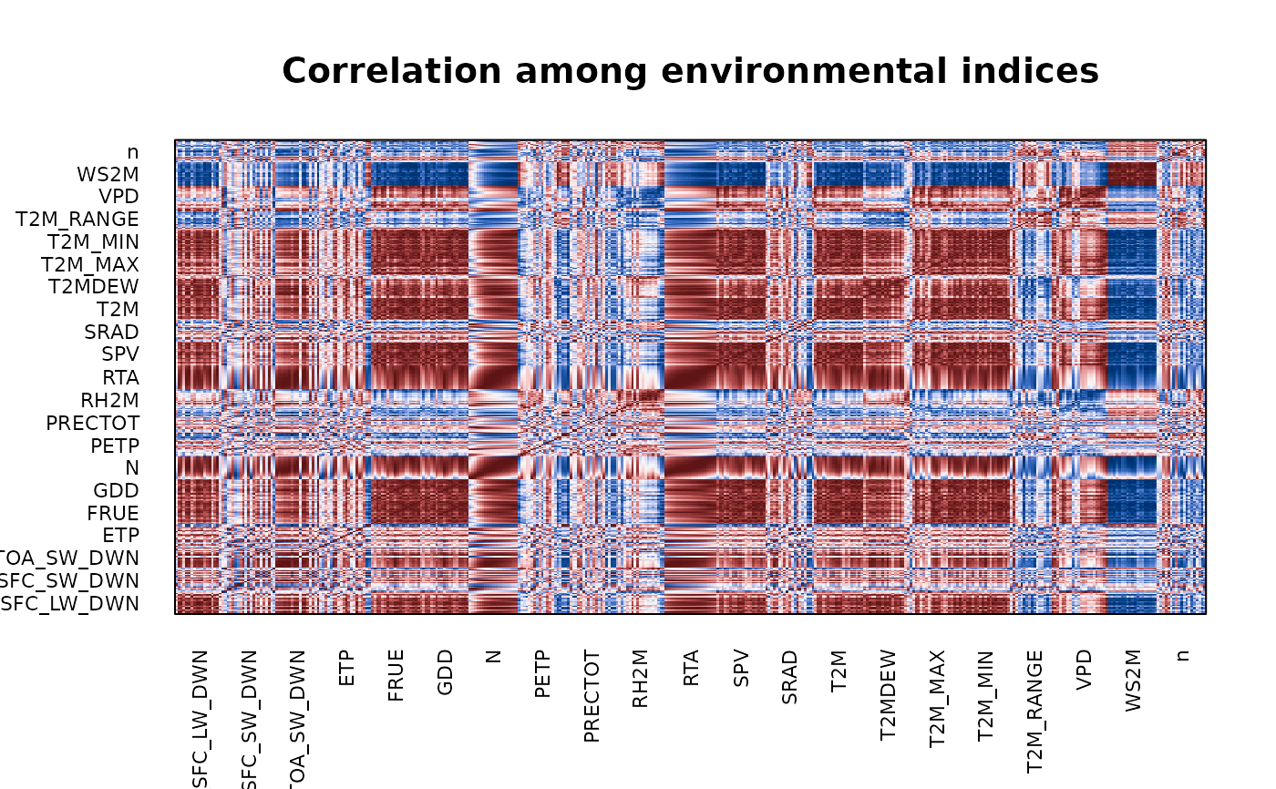
Pearson correlation among all environmental indices, as in Fig. 1b of Della Coletta et al. (2023), which motivated the dimensionality reduction: the 867 indices were highly correlated.
Usage
env_cor_heatmap(
  W,
  order = c("factor", "interval", "none"),
  max.index = 400L,
  title = "Correlation among environmental indices",
  verbose = TRUE
)
Arguments
- W
matrix. Environment x index matrix from
env_indices.- order
character. Column ordering:
"factor"(default, groups all intervals of a factor together, giving the block structure of Fig. 1b),"interval"(chronological across factors) or"none".- max.index
integer. Guard against enormous plots; if the matrix has more columns than this, a regularly spaced subset is shown. Default 400.
- title
character. Plot title.
- verbose
boolean. If
TRUE(default) prints a progress banner.
Details
The mean absolute off-diagonal correlation is printed as a one-number summary of how redundant the index set is – the quantity that justifies running a PCA at all.
Examples
# \donttest{
W <- env_indices(maizeWTH, end.day = 130)
#> ---------------------------------------------------------------
#> env_indices -- builds interval-resolved environmental indices
#> Last updated at 09/27/2026
#> ---------------------------------------------------------------
#> ------------------------------------------------------------
#> env_indices(): 5 environments x 21 factors x 44 intervals = 924 indices
#> interval width : 3 day(s), days 1..130
#> discarded : 106 record(s) outside 1..130
#> ------------------------------------------------------------
R <- env_cor_heatmap(W)
#> ---------------------------------------------------------------
#> env_cor_heatmap -- plots correlation among environmental indices
#> Last updated at 09/27/2026
#> ---------------------------------------------------------------
#> Showing 400 of 924 indices (raise 'max.index' to see more).
#> Mean |r| among indices: 0.544 (high values justify the PCA)
 # }