PCA of Interval-Resolved Environmental Indices

Runs prcomp on the environment x index matrix, as in Della Coletta et al. (2023), and returns scores, loadings and variance explained in a form the plotting functions in this module can consume.

Usage

env_pca(
  W,
  center = TRUE,
  scale. = TRUE,
  rank. = NULL,
  drop.constant = TRUE,
  verbose = TRUE
)

Arguments

W: matrix. Environment x index matrix, typically from env_indices.
center: boolean. Centre the indices. Default TRUE.
scale.: boolean. Scale the indices to unit variance. Default TRUE; see Details for why this differs from a bare prcomp call.
rank.: integer or NULL. Maximum number of PCs to compute. NULL (default) computes all available, which is min(nrow - 1, ncol).
drop.constant: boolean. If TRUE (default) indices with zero variance are removed before the PCA rather than producing NaN under scaling.
verbose: boolean. Print a summary. Default TRUE.

Value

A list of class "env_pca":

scores: environment x PC matrix (prcomp$x)
loadings: index x PC matrix (prcomp$rotation)
variance: data.frame with PC, sd, prop, cum
prcomp: the underlying prcomp object
dropped: indices removed as constant
meta: data.frame mapping each index to its factor, interval and day

Details

Scaling. The paper reports only that prcomp was used. Because the 17 factors are on incomparable scales – radiation in MJ/m2/day, precipitation in mm, FRUE unitless in [0,1] – an unscaled PCA is dominated by the highest-variance factor and the leading PCs largely describe that one variable. scale. = TRUE is therefore the default here. Set scale. = FALSE for a covariance-matrix PCA.

Rank. With $q$ environments and $k \gg q$ indices, at most $q - 1$ PCs carry variance. With the 9 environments of the paper that is 8, so the reported "ninth PC" explaining $<0.01\%$ is effectively numerical noise. Expect very few informative PCs unless you have many environments.

Examples

# \donttest{
data("maizeWTH")
W  <- env_indices(maizeWTH, end.day = 130)
#> ---------------------------------------------------------------
#> env_indices -- builds interval-resolved environmental indices
#> Last updated at 09/27/2026
#> ---------------------------------------------------------------
#> ------------------------------------------------------------
#> env_indices(): 5 environments x 21 factors x 44 intervals = 924 indices
#>   interval width : 3 day(s), days 1..130
#>   discarded      : 106 record(s) outside 1..130
#> ------------------------------------------------------------
pc <- env_pca(W)
#> ---------------------------------------------------------------
#> env_pca -- runs PCA on the environmental index matrix
#> Last updated at 09/27/2026
#> ---------------------------------------------------------------
#> ------------------------------------------------------------
#> env_pca(): 5 environments x 924 indices
#>   informative PCs: 4 (= n.env - 1)
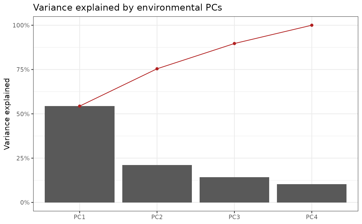
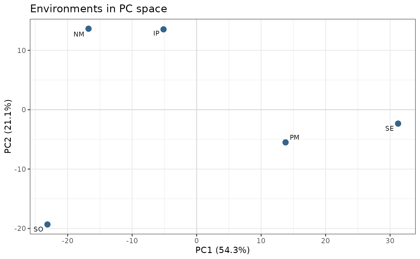
#>   PC1 54.3%, PC2 21.1%, cumulative 75.4%
#> ------------------------------------------------------------
head(pc$variance)
#>    PC       sd      prop       cum
#> 1 PC1 22.40939 0.5434858 0.5434858
#> 2 PC2 13.95208 0.2106715 0.7541572
#> 3 PC3 11.47995 0.1426290 0.8967863
#> 4 PC4  9.76573 0.1032137 1.0000000
env_pca_scree(pc)
#> ---------------------------------------------------------------
#> env_pca_scree -- plots variance explained per PC
#> Last updated at 09/27/2026
#> ---------------------------------------------------------------

env_pca_biplot(pc)
#> ---------------------------------------------------------------
#> env_pca_biplot -- plots environments in PC space
#> Last updated at 09/27/2026
#> ---------------------------------------------------------------

# }