Scree Plot of Environmental PCA

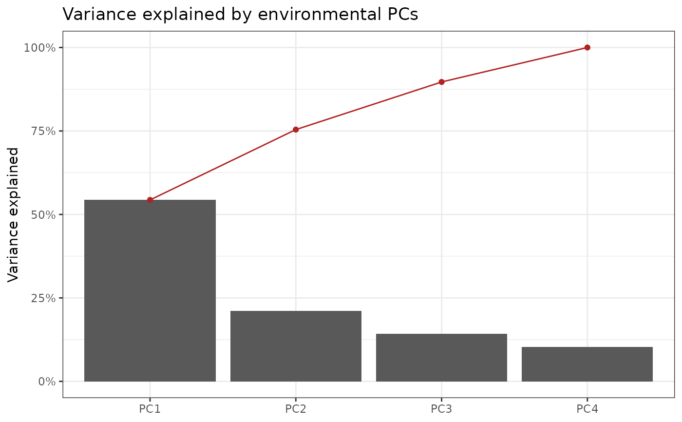
Plots the proportion of variance explained per PC, the visualisation the paper used to decide how many PCs to retain.

Usage

env_pca_scree(
  x,
  n.pc = NULL,
  cumulative = TRUE,
  title = "Variance explained by environmental PCs",
  verbose = TRUE
)

Arguments

x

an env_pca object.

n.pc

integer. How many PCs to show. Default min(15, available).

cumulative

boolean. Overlay the cumulative proportion. Default TRUE.

title

character. Plot title.

verbose

boolean. If TRUE (default) prints a progress banner.

Value

A ggplot object when ggplot2 is available (invisibly), otherwise NULL after drawing a base plot.

See also

env_pca

Examples

# \donttest{
pc <- env_pca(env_indices(maizeWTH, end.day = 130))
#> ---------------------------------------------------------------
#> env_pca -- runs PCA on the environmental index matrix
#> Last updated at 09/27/2026
#> ---------------------------------------------------------------
#> ---------------------------------------------------------------
#> env_indices -- builds interval-resolved environmental indices
#> Last updated at 09/27/2026
#> ---------------------------------------------------------------
#> ------------------------------------------------------------
#> env_indices(): 5 environments x 21 factors x 44 intervals = 924 indices
#>   interval width : 3 day(s), days 1..130
#>   discarded      : 106 record(s) outside 1..130
#> ------------------------------------------------------------
#> ------------------------------------------------------------
#> env_pca(): 5 environments x 924 indices
#>   informative PCs: 4 (= n.env - 1)
#>   PC1 54.3%, PC2 21.1%, cumulative 75.4%
#> ------------------------------------------------------------
env_pca_scree(pc)
#> ---------------------------------------------------------------
#> env_pca_scree -- plots variance explained per PC
#> Last updated at 09/27/2026
#> ---------------------------------------------------------------

# }