
Correlate Environmental PCs with a Per-Environment Variable
Source:R/env_dissection.R
env_pc_associate.RdPearson correlation between each environmental PC and an external per-environment quantity – in the paper, module eigenmarkers; equally, a trait mean, heritability or predictive ability per environment. P-values are FDR-adjusted across PCs, as in the paper.
Arguments
- x
an
env_pcaobject.- y
numeric vector or matrix. One value (or column of values) per environment. Names, or rownames, are matched against the environments in
x.- n.pc
integer. How many PCs to test. Default
min(9, available), 9 being the paper's choice.- method
character. Correlation method passed to
cor.test. Default"pearson".- p.adjust
character. Multiple-testing correction. Default
"BH"(Benjamini-Hochberg), as in the paper.- verbose
boolean. Report the strongest association. Default
TRUE.
Details
Power warning. With \(q\) environments each correlation has \(q - 2\) degrees of freedom. At the paper's \(q = 9\) even \(r = 0.86\) gives an unadjusted \(p \approx 0.003\), and a handful of PCs tested against a handful of modules exhausts the evidence quickly. Treat these associations as hypothesis- generating, not confirmatory, and prefer many environments.
FDR does not cover module selection. The adjustment applied here accounts for testing several PCs. It does not account for the eigenmarker being PC1 of a module that was itself chosen by clustering the same effect matrix. That selection inflates correlations and is invisible to any p-value computed from the observed data. See the worked example below for a permutation check, and for a demonstration that the permutation check is itself insufficient.
Examples
# \donttest{
pc <- env_pca(env_indices(maizeWTH, end.day = 130))
#> ---------------------------------------------------------------
#> env_pca -- runs PCA on the environmental index matrix
#> Last updated at 09/27/2026
#> ---------------------------------------------------------------
#> ---------------------------------------------------------------
#> env_indices -- builds interval-resolved environmental indices
#> Last updated at 09/27/2026
#> ---------------------------------------------------------------
#> ------------------------------------------------------------
#> env_indices(): 5 environments x 21 factors x 44 intervals = 924 indices
#> interval width : 3 day(s), days 1..130
#> discarded : 106 record(s) outside 1..130
#> ------------------------------------------------------------
#> ------------------------------------------------------------
#> env_pca(): 5 environments x 924 indices
#> informative PCs: 4 (= n.env - 1)
#> PC1 54.3%, PC2 21.1%, cumulative 75.4%
#> ------------------------------------------------------------
## Trait mean per environment
ybar <- tapply(maizeYield$value, maizeYield$env, mean)
env_pc_associate(pc, ybar)
#> ---------------------------------------------------------------
#> env_pc_associate -- correlates PCs with an external variable
#> Last updated at 09/27/2026
#> ---------------------------------------------------------------
#> Strongest: y1 ~ PC2, r = -0.93, p = 0.0243, FDR p = 0.097 (n = 5)
#> Note: n = 5 environments. Low power; treat as hypothesis-generating.
#> column PC r p p.adj n
#> 1 y1 PC2 -0.9252402 0.02426079 0.09704317 5
#> 2 y1 PC4 -0.3163203 0.60406959 0.83213929 5
#> 3 y1 PC3 -0.1624467 0.79407975 0.83213929 5
#> 4 y1 PC1 0.1322238 0.83213929 0.83213929 5
# }
# \donttest{
## ----------------------------------------------------------------------
## WORKED EXAMPLE: marker effect networks -> eigenmarkers -> environmental PCs
##
## The full analysis chain of Della Coletta et al. (2023), on simulated data
## where the answer is known in advance so the method can be checked.
##
## Planted truth:
## module A markers respond to mid-season TEMPERATURE
## module B markers respond to late-season PRECIPITATION
## module C markers have real but environment-INDEPENDENT effects
## ----------------------------------------------------------------------
## --- 0. Simulate markers, weather and phenotypes ---------------------
set.seed(2026)
n.gid <- 160
n.marker <- 90
n.env <- 20
envs <- paste0("E", seq_len(n.env))
drivers <- scale(matrix(rnorm(n.env * 2), n.env, 2))
rownames(drivers) <- envs
M <- scale(matrix(rbinom(n.gid * n.marker, 2, 0.5), n.gid, n.marker))
dimnames(M) <- list(paste0("G", seq_len(n.gid)),
paste0("m", seq_len(n.marker)))
beta <- matrix(0.2, n.marker, n.env)
beta[1:30, ] <- rep(0.2 + 0.3 * drivers[, 1], each = 30)
beta[31:60, ] <- rep(0.2 + 0.3 * drivers[, 2], each = 30)
signal <- M %*% beta
Y <- signal + matrix(rnorm(length(signal), sd = 0.3), n.gid, n.env)
dimnames(Y) <- list(rownames(M), envs)
wth <- expand.grid(daysFromStart = 1:151, env = envs)
ie <- match(wth$env, envs)
day <- wth$daysFromStart
wth$T2M <- 22 + 4 * sin(pi * day / 151) +
3 * drivers[ie, 1] * (day >= 50 & day <= 100) +
rnorm(nrow(wth), sd = 0.5)
wth$PRECTOT <- exp(1 + 0.6 * drivers[ie, 2] * (day >= 100) +
rnorm(nrow(wth), sd = 0.1))
## --- 1. Marker effects per environment (RR-BLUP) ----------------------
## Solve via the n x n system: with p markers >> n genotypes this is far
## cheaper than the p x p form and gives the same ridge solution.
rrblup_effects <- function(y, Z, h2 = 0.5) {
yc <- as.numeric(y) - mean(y)
lambda <- ncol(Z) * (1 - h2) / h2
a <- solve(tcrossprod(Z) + lambda * diag(nrow(Z)), yc)
as.numeric(crossprod(Z, a))
}
beta.hat <- sapply(colnames(Y), function(e) rrblup_effects(Y[, e], M, h2 = 0.55))
dimnames(beta.hat) <- list(colnames(M), colnames(Y))
## --- 2. Marker effect network -> modules ------------------------------
## Markers whose effects do not VARY across environments cannot covary with
## anything; screening them out first avoids NA correlations and spurious
## modules. The paper used WGCNA; this is the same idea in base R.
eff.sd <- apply(beta.hat, 1, sd)
Bk <- beta.hat[eff.sd > quantile(eff.sd, 0.35), , drop = FALSE]
adj <- abs(cor(t(Bk)))^6 # soft-thresholding power
mods <- cutree(hclust(as.dist(1 - adj), method = "average"), h = 0.92)
mods <- mods[mods %in% as.integer(names(table(mods))[table(mods) >= 15])]
## --- 3. Eigenmarkers --------------------------------------------------
## PC1 of a module's effect profiles, the analogue of a WGCNA module
## eigengene. Sign is arbitrary in PCA, so orient it deterministically --
## otherwise a module can flip between runs and reverse every downstream
## correlation.
eigenmarker <- function(B.mod) {
X <- scale(t(B.mod))
em <- prcomp(X, center = FALSE, scale. = FALSE)$x[, 1]
if (mean(cor(em, X)) < 0) em <- -em
em
}
ids <- sort(unique(mods))
EM <- sapply(ids, function(m) eigenmarker(Bk[names(mods)[mods == m], , drop = FALSE]))
dimnames(EM) <- list(colnames(beta.hat), paste0("ME", ids))
## --- 4. Environmental PCA and association -----------------------------
W <- env_indices(wth, interval = 3, end.day = 151,
statistic.by = c(PRECTOT = "sum"))
#> ---------------------------------------------------------------
#> env_indices -- builds interval-resolved environmental indices
#> Last updated at 09/27/2026
#> ---------------------------------------------------------------
#> ------------------------------------------------------------
#> env_indices(): 20 environments x 2 factors x 51 intervals = 102 indices
#> interval width : 3 day(s), days 1..151
#> ------------------------------------------------------------
pc <- env_pca(W)
#> ---------------------------------------------------------------
#> env_pca -- runs PCA on the environmental index matrix
#> Last updated at 09/27/2026
#> ---------------------------------------------------------------
#> ------------------------------------------------------------
#> env_pca(): 20 environments x 102 indices
#> informative PCs: 19 (= n.env - 1)
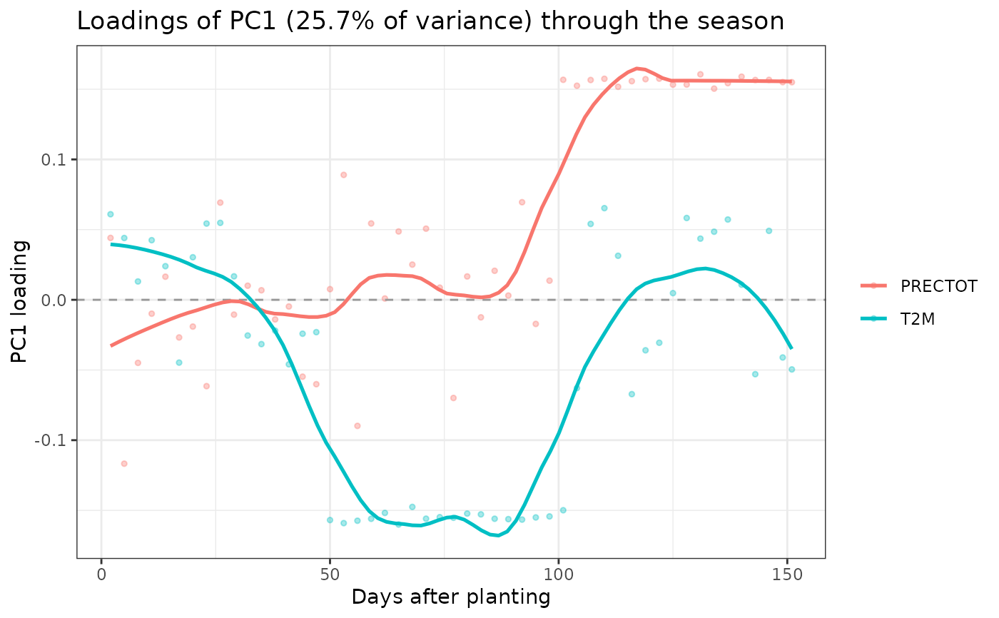
#> PC1 25.7%, PC2 16.4%, cumulative 42.1%
#> ------------------------------------------------------------
assoc <- env_pc_associate(pc, EM, n.pc = 9, p.adjust = "BH")
#> ---------------------------------------------------------------
#> env_pc_associate -- correlates PCs with an external variable
#> Last updated at 09/27/2026
#> ---------------------------------------------------------------
#> Strongest: ME1 ~ PC1, r = -0.77, p = 7.77e-05, FDR p = 0.0014 (n = 20)
head(assoc)
#> column PC r p p.adj n
#> 1 ME1 PC1 -0.76768107 0.0000776952 0.001398514 20
#> 2 ME2 PC1 0.73762697 0.0002058673 0.001852806 20
#> 3 ME1 PC2 -0.62673494 0.0031054106 0.018632464 20
#> 4 ME2 PC2 -0.60348651 0.0048437536 0.021796891 20
#> 5 ME2 PC4 -0.12352845 0.6038587012 0.982526789 20
#> 6 ME2 PC5 -0.09614311 0.6867892239 0.982526789 20
## --- 5. Name the drivers of an associated PC (paper Fig. 6c) ----------
k <- as.integer(sub("PC", "", assoc$PC[1]))
L <- data.frame(factor = pc$meta$factor, day = pc$meta$day,
loading = pc$loadings[, k])
sort(tapply(abs(L$loading), L$factor, mean), decreasing = TRUE)
#> T2M PRECTOT
#> 0.08056294 0.07779317
env_loading_curve(pc, pc = k)
#> ---------------------------------------------------------------
#> env_loading_curve -- plots seasonal PC loading curves
#> Last updated at 09/27/2026
#> ---------------------------------------------------------------
 ## --- 6. Permutation null, and why it is NOT enough --------------------
## Permuting environment labels of the eigenmarker breaks the
## environment<->module link while preserving both structures.
perm.max <- replicate(500, {
EMp <- EM[sample(nrow(EM)), , drop = FALSE]
rownames(EMp) <- rownames(EM)
max(abs(env_pc_associate(pc, EMp, n.pc = 9, verbose = FALSE)$r))
})
quantile(perm.max, 0.95) # compare observed |r| with the permutation null
#> 95%
#> 0.6557894
## A spurious module can pass both FDR adjustment and this permutation test.
## The permutation preserves the module definitions, so it cannot detect a
## module that was spuriously assembled in the first place. Guard against
## this with module stability across resampled genotypes, or by requiring
## an independent set of environments -- not with permutation alone.
# }